Analyzing and Predicting Policyholder Behavior at Policy-Level with Machine Learning: Part 2— Machine Learning Model’s Architecture, Performance, and Applications in Experience Studies and Assumption Setting
By Shaio-Tien Pan and Jack Liu
The Financial Reporter, November 2024

This is the second of a two-part article. Part 1 (September 2024 issue of The Financial Reporter) discussed the limitations of traditional experience studies and assumption setting methods, and briefly introduced an alternative machine learning approach to analyze and model policyholder behavior. Part 2 describes the machine learning model’s architecture, performance and applications in detail.
Model Architecture
The model includes two modules: A recurrent neural network (RNN) and a feed forward neural network (FFNN). The RNN takes the policy's sequence of transactions as input, and outputs an embedding, or a representation of the policyholder's historical transactions. The embedding is then concatenated with the other policy data and together fed through the FFNN, which outputs a prediction of the policyholder's action over the next period. The embedding effectively transforms the time-series transactional data {τ1 , τ 2,…, τt-1} into information in tabular form that can be easily concatenated with other tabular data Xstatic and Xt for downstream tasks. Figure 1 illustrates the architecture and learning process.
Figure 1
Model Architecture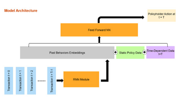
We utilized multi-task learning to reflect the different types of transactions a policyholder can make. Specifically for our variable annuity (VA) guaranteed lifetime withdrawal benefit (GLWB) example, our FFNN consists of a shared sub-network and two type-specific (partial withdrawal and lapse) sub-networks via a multi-head architecture.[1] In effect, our model is trained to learn and predict withdrawal amount and lapse simultaneously. This turns out to be another major benefit of our approach over traditional actuarial methods, which tend to treat partial withdrawals and lapses as separate assumptions and study them independently. Yet industry experience consistently indicates that partial withdrawals and lapse behaviors are intimately correlated: Policyholders with a history of excess or ad hoc withdrawals have displayed higher propensity to lapse, while people who are efficient (i.e., taking close to the maximum allowed amount) or systematic in their withdrawals are unlikely to surrender. Our multi-task learning model would automatically and elegantly capture such interrelationships. In addition, by using just one learning model for multiple assumptions, our approach offers efficiency gain.
Finally, to generate transactions over multiple periods in the future, we can recursively generate the next policyholder action, append the generated transaction to the transaction sequence, feed the updated sequence through the model again to generate the next transaction, and so on. We rely on the actuarial model to project future market returns and time-dependent variables (Xt for t = T+1, T+2,…) such as account value. We will discuss how to integrate our machine learning model and the actuarial valuation model in the Application to Actuarial Valuation section.
Experimental Results
We evaluated our custom machine learning model using a large VA GLWB dataset that consisted of more than 10 years of experience. Our model was trained to predict 2022 partial withdrawals and lapses using experience up to 2021. For simplicity, we limited our experiment to policies that have taken withdrawals previously (i.e., policies with at least one withdrawal transaction prior to 2022). We trained the model using 80% of the data, and then compared the performance of the model on the test set against a benchmark assumption set developed using the typical traditional actuarial approach.[2]
We observe that our model significantly outperforms the benchmark actuarial assumptions. As shown in Figure 2, relative to the benchmark the mean absolute error (MAE) of our model’s partial withdrawal predictions is 55.2% lower, while on lapse predictions our model achieves an area under the receiver operating characteristics curve (a.k.a., area under the curve, or AUC ) that is 0.221 higher. These results suggest that the model demonstrates a strong ability to differentiate policyholders and make reasonable predictions at the individual policy level.
Figure 2
Model Performance and Comparison to Benchmark Assumptions 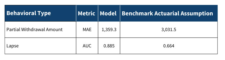
It turns out that our model performs better on many aggregate actual-to-expected (A/E) metrics too. For example, for partial withdrawals the model achieves an overall A/E of 99.4%, compared to 98.4% for the benchmark assumption. Upon further analysis, we believe there are two main reasons for the outperformance: Our model is better equipped to capture 1) policyholders are becoming more efficient, and 2) inefficient policyholders tend to lapse more, so the portion of efficient withdrawers increases over time. By treating the sequence of prior transactions as a time series and making predictions at the policy level, our model is more reactive to changes in behaviors and the shift in in-force mix. In contrast, the benchmark assumption is based on average aggregate experience over five years and will tend to lag behind any trend.
Policyholder Representation
In our proposed model, the final hidden state (basically a vector of numerical values) of the RNN is a policyholder embedding representation that characterizes a policy’s prior behaviors. During training the RNN learns to capture the salient and relevant transactional patterns and encode that information in the embedding vector. In addition to being a feature engineering technique to convert time-series data into tabular, embedding can also be viewed as a method to place millions of heterogenous policyholders in a low dimensional space based on their transactional behaviors. Policyholders with similar behaviors are expected to be closer together in the resulting embedding space. Figure 3 shows the resulting policyholder embeddings projected into a two-dimensional space using the t-SNE algorithm,[3] with each point on the graph representing a particular policy. The embeddings are based on transactions up to 2021, and we color-code each point based on the policy’s 2022 withdrawal amount classified into a few categories.
Figure 3
Visualization of Policyholder Embeddings in 2D, Color Coded Based on Withdrawal Behavior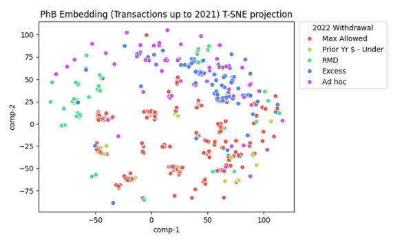
We observe that the colors are well clustered in the graph. This implies that the model can extract meaningful patterns from the transaction data, and that the resulting embeddings are predictive of future withdrawal behaviors. Also, note that the more systematic withdrawers (i.e., people taking the maximum allowed amount, or the same amount as prior year, or the required minimum distribution (RMD) amount) are concentrated in the lower left half of the graph, while policies taking excess withdrawals or displaying other ad-hoc behaviors tend to gravitate more toward the upper right.
Figure 4 shows that if we color-code the points by 2022 surrender behaviors instead, there are more lapses among policies in the upper right (i.e., the excess and ad-hoc withdrawers) as expected. Conversely, systematic withdrawers seldom lapse.
Figure 4
Visualization of Policyholder Embeddings in 2D, Color Coded Based on Lapse Behavior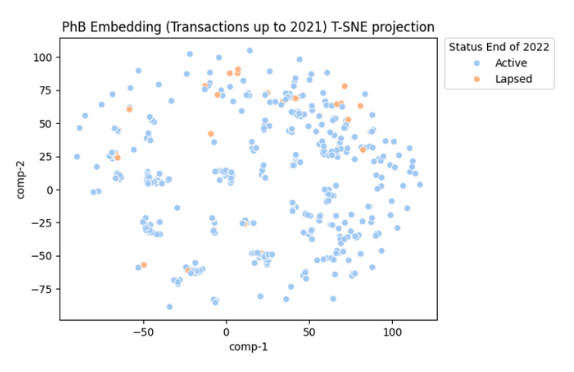
The policyholder embeddings have stand-alone values beyond our model. They can be used to segment policyholders or to infer policyholders’ hidden attributes, which may have marketing, in-force management, and other applications.
Application to Actuarial Valuations
Since our proposed model analyzes experience data and makes predictions at the level of individual policies, it allows actuaries to effectively set policy-level assumptions in their valuation models. While that may sound operationally challenging and impractical, it is actually simple and feasible. The trained machine learning model will essentially replace the various assumption tables and formulas in the actuarial model. During run-time, the actuarial model would at each time step emit the policy state data to the machine learning model and receive in return the predicted policyholder behavior (e.g., the withdrawal amount and lapse probability). There shouldn’t be much of a difference in run-time, as inferencing a machine learning model is no more computationally intensive than executing a series of table lookups and calculating a formulaic dynamic lapse rate that the actuarial model would otherwise do currently. On the other hand, the machine learning approach could greatly simplify the current laborious and often subjective experience studies and assumption setting process, since the training of the machine learning model can be largely automated. In addition, as mentioned previously, one model can be leveraged for multiple policyholder behavioral assumptions. Policy-level assumptions also improve the accuracy of liability valuation, which is especially valuable for M&A and reinsurance transactions.
One potential disadvantage of the machine learning approach is that the model may seem opaque and more difficult to explain. I believe education and having a robust model validation framework suitable for AI models are especially important and can help mitigate these concerns.
Conclusion
In this article, I have introduced a novel machine learning-based model suitable for analyzing and predicting policyholder behavior. The model offers many advantages over the traditional actuarial approach to experience studies and assumption setting, including the ability to produce policy-level assumptions that improves liability estimates, projecting multiple assumptions while capturing the interrelationships between them, and creating policyholder embedding representations that are useful for segmentations.
Statements of fact and opinions expressed herein are those of the individual authors and are not necessarily those of the Society of Actuaries, the newsletter editors, or the respective authors’ employers.
Shaio-Tien Pan, FSA, MAAA, is a director at PwC. He can be reached at shaio-tien.pan@pwc.com.
Jack Liu, FSA, MAAA, is a senior manager at PwC. He can be reached at rongjia.liu@pwc.com.
Endnotes
[1] In multi-task learning, a multi-head architecture refers to a neural network that consists of common hidden layers with shared parameters for all tasks, and several task-specific layers toward the end of the model.
[2] For partial withdrawals the assumption is set based on the average experience over the past five years and varies by tax status and age. For lapse, the assumption is set based on the average experience over the past five years and varies by product, policy year, surrender charge period, policy size, and in-the-moneyness.
[3] t-distributed stochastic neighbor embedding (t-SNE) is a statistical method for visualizing high-dimensional data, such that data points that are similar or close in the original (high dimensional) space are expected to stay in proximity in two-dimensional space with high probability.